This module is based on the following documentation :

Seurat v4 R package

Hao Y, Hao S, Andersen-Nissen E, et al. Integrated analysis of multimodal single-cell data. Cell. 2021;184(13):3573-3587.e29. doi:10.1016/j.cell.2021.04.048
* https://satijalab.org/seurat/articles/get_started.html
* https://htmlpreview.github.io/?https://github.com/satijalab/seurat.wrappers/blob/master/docs/harmony.html

Guidelines for scRNA-seq analysis and integration of multiple samples

Luecken MD, Theis FJ. Current best practices in single-cell RNA-seq analysis: a tutorial. Mol Syst Biol. 2019;15(6):e8746. Published 2019 Jun 19. doi:10.15252/msb.20188746
* https://pubmed.ncbi.nlm.nih.gov/31217225/

Luecken MD, Büttner M, Chaichoompu K, et al. Benchmarking atlas-level data integration in single-cell genomics. Nat Methods. 2022;19(1):41-50. doi:10.1038/s41592-021-01336-8
* https://pubmed.ncbi.nlm.nih.gov/34949812/

This module require to load the following environment of R packages :

source("/home/truchi/Starter_pack.R")

Informations about the demo dataset :

The demo dataset is a collection of 18 public 10X Genomics Chromium samples (GSE151374) of control (n=6) or bleomycin-treated mice lungs (n=12), collected after 7 or 14 days following treatment. Half of bleomycin-treated mice were also treated with Nintedanib, an anti-fibrotic drug (see associated publication).

Notes

Sequencing multiple samples is necessary to obtain robust observations on the organization of a physiological tissue or on variations induced by an experimental condition. It is also needed when studying dynamic processes, such as responses to a treatment, the evolution of a pathology, or development and differentiation pathways, which require monitoring over time.

Due to the technical uncertainties involved in collecting, preparing and sequencing the RNA from each sample, data obtained from different experiments generally show a high degree of unwanted variability which intermingles with the biological signal. This technical variability, summarized under the term "batch effect", is reflected both in the overall RNA quantification and other transcriptomic signatures, such as ectopic cellular-stress. Without correction and despite data normalization, batch effect is likely to bias biological conclusions deduced from a sample-specific phenomenon. However, correcting batch effect is a complex task when considering different experimental conditions, as it must not erase the biological signal of interest.

In this context, successful data integration guarantees correction of the batch effect, while preserving the biological variability of the dataset in a computationnaly effective manner. The performances of dozens of integration tools proposed in the literature have been compared according to these same criteria. They appear highly dependent on the total number of samples to integrate and the degree of biological and technical variability between samples. For simple tasks, i.e. integrating less than 100k cells from homogeneously-collected samples, R packages such as Harmony or FastMNN showed the best results. For more complex tasks, python packages such as scANVI or scVI are recommended.

In this vignette, we will run Harmony from Seurat v4 extension provided in the seurat-wrapper R package.

1. Pre-processing

1.1 Read raw count matrix

The first step is to read the raw count matrix for each sample. Depending on the dataset, you can encounter different cellranger/STAR outputs, such as subdirectories containing 3 files (matrix.mtx, features.tsv, barcodes.tsv) or .h5 files.

# Change your working directory to the repertory containing all cell ranger outputs
dr <- c("/my/directory/scRNAseq_data/")
setwd(dr)

As a example, we load a .h5 file as a dgCMatrix (a class of compressed sparse numeric matrices), rename their column names and then transform it to a seurat object. By adding a unique prefix to the column names of each sample, we prevent redondant barcodes names events that can happened when integrating independantly sequenced samples. We also immediately eliminate genes expressed in less than 10 cells and cells containg less than 500 uniquely detected genes.

PBS_None_7_r1 <- Read10X_h5(filename = "Control_None_7_r1.h5") 
colnames(PBS_None_7_r1) <- paste0("PBS_None_7_r1.",colnames(PBS_None_7_r1))
PBS_None_7_r1 <- CreateSeuratObject(PBS_None_7_r1,min.cells = 10,min.features = 500)

1.2 Perform quality control for each sample

Then, we filtered out barcodes more likely to correspond to degraded cells, characterized by a low UMI-content, a poor number of uniquely detected genes, or a high fraction of counts corresponding to mitochondrial transcripts. Those features are indeed interpreted as the result of degradation of cell membrane integrity, resulting in the loss of cytoplasmic RNA while mitochondrial and nuclear transcripts are preserved. Cells considered to be of poor quality are eliminated by applying arbitrary thresholds based on the distribution of these 3 metrics over the whole dataset. Cells displaying a too high UMI content can also be discared, as they could also biais the analysis. However, some flexibility is recommended in setting these thresholds, to avoid excluding cell types or states characterized by low transcriptomic content or higher levels of mitochondrial transcripts. More generally, quality control should be an iterative process in which the initial parameters are adjusted in the light of the effects observed on the final clustering of cells. Typically, cells grouped according to their UMI content, their high proportion of mitochondrial transcripts, or marked by a stress signature, rather than by the expression of biologically relevant transcripts, are to be eliminated a posteriori.

mito.genes <- grep(pattern = "^mt-", x = rownames(PBS_None_7_r1@assays$RNA), value = TRUE)
percent.mito <- Matrix::colSums(PBS_None_7_r1@assays$RNA[mito.genes, ])/Matrix::colSums(PBS_None_7_r1@assays$RNA)
PBS_None_7_r1[['percent.mito']] <- percent.mito
VlnPlot(PBS_None_7_r1, features = c("nFeature_RNA", "nCount_RNA","percent.mito"),pt.size = 0.1, ncol=3,sort =T)
dim(PBS_None_7_r1@assays$RNA)
PBS_None_7_r1 <- subset(PBS_None_7_r1, cells = PBS_None_7_r1@meta.data %>% filter(nCount_RNA < 20000 & percent.mito < 0.15) %>% rownames(.))
dim(PBS_None_7_r1@assays$RNA)
VlnPlot(PBS_None_7_r1, features = c("nFeature_RNA", "nCount_RNA","percent.mito"),pt.size = 0.1, ncol=3,sort =T)

1.2 Pre-process all samples iteratively

As all samples have a similar distribution of QC metrics, we just set the same thresholds in a function that pre-process all samples iteratively. It produces a list of n seurat objects, where n = the number of samples (18).

files.list <- list.files()
do_QC <- lapply(files.list, function(file){
  data <- Read10X_h5(filename = file) 
  colnames(data) <- paste0(gsub("\\..*","",file),".",colnames(data))
  data <- CreateSeuratObject(data,min.cells = 10,min.features = 500)
  dim(data)
  mito.genes <- grep(pattern = "^mt-", x = rownames(data@assays$RNA), value = TRUE)
  percent.mito <- Matrix::colSums(data@assays$RNA[mito.genes, ])/Matrix::colSums(data@assays$RNA)
  data[['percent.mito']] <- percent.mito
  dim(data@assays$RNA)
  data <- subset(data, cells = data@meta.data %>% filter(nCount_RNA < 20000 & percent.mito < 0.15) %>% rownames(.))
  dim(data@assays$RNA)
  data
}) 

Then, we merge all 18 elements of the list as a single object and add some metadata informations based on barcodes names.

aggr <- Reduce(merge,do_QC)
aggr$barcode <- colnames(aggr)
aggr$sample <- gsub("\\..*","",colnames(aggr))
aggr$condition <- ifelse(grepl("BLM",aggr$barcode),"BLM","CTRL")
aggr$treatment <- ifelse(grepl("Nintedanib",aggr$barcode),"Nintedanib","None")
aggr$time.point <- ifelse(grepl("_14_",aggr$barcode),"d14","d7")
aggr$group <- ifelse(grepl("Control",aggr$barcode),"CTRL",paste(aggr$condition,aggr$treatment,aggr$time.point,sep = "_"))
aggr$group <- factor(aggr$group,levels = c("CTRL","BLM_None_d7","BLM_Nintedanib_d7","BLM_None_d14","BLM_Nintedanib_d14"))

2. Computational integration of samples and cells clustering

2.1 Run Harmony integration

Prior to run Harmony, data must be normalized (CP10k normalization + log-transformation), scaled, and projected in PCA space.
Scaling and PCA projection are done only for the top 4000 most variable features.

aggr <- aggr %>% NormalizeData() %>% FindVariableFeatures(nfeatures = 4000) %>% ScaleData() %>% RunPCA(verbose = FALSE,npcs = 100)

To run Harmony, the column names containing the samples identities must be precised

aggr <- RunHarmony(aggr, group.by.vars = c('sample'))

2.2 Run clustering and 2D-visualization in UMAP

The aim of data pre-processing, normalization, dimension reduction and integration is to extract the biological signal that enables cells to be grouped according to their transcriptomic profiles that reflect their physiological functions and responses to stimuli.
To do so, a graph-based kNN clustering is performed on the cell distancies in the Harmony's integrated space of n components.
Only the edges of the computed graph linking each cell to its k nearest neighbors are retained.
Louvain’s graph partitioning algorithm is then used to isolate the nearest cell communities.
A resolution parameter can be increased to favor the formation of small communities, corresponding, for example, to rare cell types.
However, high resolution will tend to split large though homogeneous communities into several subsets whose distinguishing features are generally of little relevance from a biological point of view.
It is often more practical to do an over-clustering and then merge homogeneous clusters together, but it is also possible to perform a first round of coarse clustering and then subcluster each coarse cluster in order to identify smaller communauties.

aggr <- FindNeighbors(aggr, reduction = 'harmony', dims = 1:50,k.param = 20)
aggr <- FindClusters(aggr, resolution = 1)

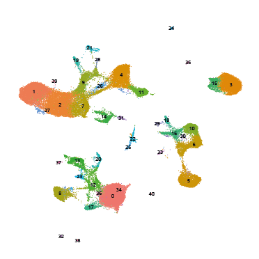
To facilitate data exploration and interpretation, cells can be represented in a 2-dimensional space where each cluster is identifiable, so as to visualize gene expression in the different clusters.
The t-SNE and UMAP methods are mathematically complex algorithms that have been rapidly adopted in bioinformatics to address the visualization problem posed by high-dimensional data.
However, it has been shown that while these representations partly reflect the topology of the initial data, the drastic reduction in dimensions is accompanied by a massive distortion of the distances between cellular transcriptome profiles. This distortion of spatial relationships applies as much to distances between neighboring cells as to distances between different clusters. Theoretically more respectful of global structures, the UMAP representation is, in reality, no more efficient. In this context, cluster shapes and distances represented in t-SNE or UMAP should never be over-interpreted.
Finally, the main advantage of UMAP over t-SNE is its speed of execution, making it the preferred method for visualizing large datasets.

aggr <- RunUMAP(aggr, reduction = 'harmony', dims = 1:50)
# visualize the cells in UMAP, colored by clusters or group
p1 <- DimPlot(object = aggr, group.by = "seurat_clusters",reduction = "umap", label=TRUE)+ ggtitle("Clusters")+NoAxes()+NoLegend()
p2 <-DimPlot(object = aggr,group.by = "group")+ ggtitle("Condition")+NoAxes()+NoLegend()
plot_grid(p2,p1,ncol = 2)